In discrete automatic control systems, the conversion of signals is not continuous but discrete in time, in level or in time and level simultaneously. Depending on this, all discrete systems can be divided into impulse, relay and digital.
Pulsed automatic control systems are characterized by the fact that the signals acting in them are sequences of equidistant pulses (with period T) whose height or duration is proportional to the values of the signals themselves at discrete instants of time (Fig. 11.17, a and b). A device that converts a continuous signal in such systems is a pulse element (see Chapter XV).
It is customary to refer to relay automatic control systems such systems in which the signal is transformed by level (Fig. 11.17, c). As already mentioned above, in such systems, a relay element is the device that converts a continuous signal (see Chapter XIV).
Fig. II.17. Types of discrete signals: a - amplitude-pulse; b - pulse-width; in - relay; d - digital (code-pulse); 1 - continuous input signal; 2 - converted output signals
Fig. II.18. (see scan) Simplified circuit of a discrete system of programmable table feed control of a milling machine
And, finally, digital automatic control systems are characterized by the fact that in them the signal is converted both in time and in level (Fig. 11.17, d). As the devices that convert signals in digital systems, converters "code-analog", "analog-code" and digital computer (see Chapter VI) are used.
In the form of the first example of a discrete automatic control system, let us consider a system of programmable feed control for one coordinate of a milling machine table. A simplified diagram of this system is shown in Fig. 11.18. It can be seen from the figure that the system consists of the following main devices: I - input; II - photoelectric analog-code converter; III - double reverse pulse counter; IV - converter "code-analog"; V - power amplifier; VI - electric stepper motor; VII - mechanical gearbox with a cylindrical gear transmission; VIII - rejki, fastened with a table of the milling machine tool.
The input device is a tape drive mechanism with a magnetic tape on which pulses are recorded for one coordinate control: on one track pulses for controlling the motion of the machine table in one direction, and on the other track in the opposite direction. From the magnetic heads 1 signals are fed to the unit 2, where they amplify and form into regular rectangular pulses. At the same time, their synchronization in block 3 is performed with pulses coming from photodiodes of the photoelectric analog-code converter (see Chapter VI). The synchronization circuit serves to exclude the possibility of information loss when the pulses from the input device and from the photoelectric converter coincide in time with the binary reversing counter (see Chapter VI).
The binary reversive counter performs the function of the comparator, where the pulses are applied to it. The counter stores any number of pulses from 0 to 128. For the zero state of the counter, a state is accepted when there are 64 pulses in it.
A "code-analog" converter (see Chapter VI) is connected to the output of the counter, converting the pulses into a direct current voltage, which enters the power amplifier. The amplifier not only amplifies the DC signal, but also provides virtually instantaneous connection in a certain sequence of the stator windings of the stepper motor (see Chapter VII). Stepper motor through the reducer ensures the movement of the rack, and therefore the feed table.
The disk with the code mask of the photoelectric converter rotates simultaneously with the shaft of the stepper motor. Code mask 7 is an alternation of transparent and opaque areas, arranged in a certain sequence. When the light flux from the light bulb 4 passes through the slit diaphragm 5, the resulting flat beam 6 passes through the transparent regions of the disc to a multi-cell photocell 8, where impulse signals are generated.
Fig. II.19. (see scan) Block diagram of a discrete system for programmable table feed control of a milling machine
As a result, pulsed signals corresponding to the angle of rotation of the disk are removed from the photocells, since different definite combinations of transparent and opaque regions correspond to different angles of rotation.
The discrete system works as follows. The control signal read from the magnetic tape passes through the electronic circuits of pulse formation and synchronization to the first input of the reversing counter. At its output, a pulse signal is formed, which is transformed into a constant voltage by the "code-analog" converter.
This voltage is amplified and enters the stator windings of the stepper motor. The stepper motor rotates and moves the machine bed by one step. At the same time, the code disk rotates. As a result, a pulse signal is formed on the photocells, which also after the formation and synchronization is fed to the second input of the reversing counter. The signal on the second input compensates the signal at the first input, and the machine bed, having moved one step, stops.
The value of one step in the system corresponds to the minimum value of the table feed of the milling machine. At the majority of modern automatic milling machines with program regulation it is 0.01-0.02 mm.
In Fig. 11.19 is a block diagram of a discrete system for programmable table feed control of a milling machine.
In the form of a second example of a discrete automatic control system, consider the tracking system of a radar station. At radar stations, the range to the target is measured by the time shift between the pulses sent by the transmitter and the pulses received by the receiver. If you measure the range to the target in meters, it will be determined by the formula
Fig. II.20. Block diagram of the tracking system of the radar range finder
Fig. II.21. Types of signals in the tracking system of the radar range finder
A block diagram of the tracking system of the radar range finder is shown in Fig. 11.20. The pulses reflected from the target (Figure 11.21) form two-polar pulses of different amplitudes at the output of the discriminator, whose constant component represents the error signal.
After the discriminator, a memory element is installed (see Chapter XV), in which each pulse value of the signal is stored until the next signal arrives. As a result, a step signal is produced in the form of a DC voltage
After that, the signal is amplified in the amplifier and fed to a stepper motor, where a signal is generated. On the motor axis, a phase shifter is supplied, feeding a sinusoidal voltage whose zero phase coincides with the moment of pulse emission by the transmitter (Figure 11.21).
The sinusoidal voltage at the output of the phase shifter is shifted by 90 ° relative to the phase. After the phase shifter, a forming element is set up, which forms the half-strokes of accompaniment in such a way that their midpoint coincides with the zero phase of the signal. These half-strokes enter the discriminator. If the middle of the reflected pulses does not coincide with the middle of the half-strokes, then at the output of the discriminator there is an error signal of such a sign that after the rotation of the phase shifter the half-strokes move, reducing the error of the error. As a result, the stepper motor rotates by an angle proportional to the distance to the target.
Ministry of Education and Science of the Russian Federation
Federal State Budget Educational Institution
higher professional education
"KUBAN STATE UNIVERSITY"
(FGBOU HPE "KubSU")
EXTENDED QUALIFICATION OF BACHELOR
Development and design of PID controllers
The work was carried out by Roman Valeryevich Presnyakov
scientific adviser
dr. fiz.-mat. Sciences, Professor
E.N. Tumayev
Standard controller
cand. fiz.-mat. Sci., Associate Professor AA Martynov
Krasnodar 2015
abstract
Graduation qualification work 83 pp., 29 Fig., 42 sources.
PID ADJUSTMENT, BUILT-IN SYSTEMS, MICROCONTROLLERS, SOFTWARE MODULES, MSP430, INTERRUPTIONS
The object of investigation of the final qualifying work is the study of the general principles of the construction of proportional-integral-differential technological regulators and the design of an algorithm for temperature controllers based on cheap microcontrollers MSP430 (Texas Instruments). In work the review of means of modern microcontrollers and principles of their work is carried out.
The analysis of problems of hardware and software implementation of technological microprocessor regulators is carried out. Recommendations are given on the design of microprocessor measuring and control devices and the creation of software for embedded systems. An embodiment of the PID-controller algorithm is proposed. A distinctive feature is the use of algorithms that exclude the use of floating-point numbers.
Notations and abbreviations
Introduction
1. Principles of creating PID regulators
1 General questions of implementation of PID controllers
2 Differential node of the PID controller
3 Integral node of the PID controller. Integral saturation
4 Stability of the system. Nyquist Criterion
Sensitivity functions. The equation of the digital pid controller
1 Sensitivity functions. Robustness. Impulsive switching of control modes
2 The discrete form of the regulator. The equation of the digital PID controller
Quality of regulation
1 Weakening the influence of external disturbances. Quality criteria
Adjustment of the parameters of the regulator. basic principles
1 Select the controller parameters. Manual and Automatic settings
Embedded Programming
1 General principles for the development of embedded systems
2 Stages of creating software for embedded systems
3 Hierarchy of executable code in embedded systems
Algorithm of the created software
1 Description of the algorithm of the PID-temperature controller based on the microcontroller MSP430F149
Conclusion
List of sources used
Notations and abbreviations
regulator temperature microcontroller
Microcontroller PID algorithm Proportional-integral-differential algorithm HALhardware abstraction layer IDEIntegrated development environment PWM-pulse modulation PLC programmable logic controller SCADAsupervisory control and data acquisition SPIserial peripheral interface (API) APIapplication programming interface (application programming interface) ARMautomated workplaceProgramming software
INTRODUCTION
Control of technological processes with the help of regulators working in the proportional-integral-differential law (PID regulators) allows to maintain the required technological value with a sufficiently high accuracy and acceptable noise immunity to external disturbing effects. Modern PID-controllers are implemented as a software module SCADA-system executable on the workstation (APM) or programmable logic controller (PLC), and as separate technological regulators located on local and central control cabinets. As the basic elements of information processing and management, microprocessors with limited functionality are often used, which leads to a problem of lack of hardware resources and a rise in the cost of the system.
The purpose of this work is to review the principles of constructing proportional-integral-differential regulators and to develop, based on the review, the principles of creating a PID temperature controller.
When creating a temperature PID controller, a programmable microprocessor technological measuring regulator F0303.2 was used based on the MSP430F149 microcontroller, MSP-FET430UIF programmer, P3003 voltage comparator with a voltage range from 10 nV to 11.111110 V and accuracy class 0.0005. The microcontroller program was created in the integrated development environment of IAR Embedded Workbench for MSP430. 6. Technical documentation was obtained on the site of the microcontroller manufacturer.
For the full implementation of PID regulation in a microprocessor device, the following subsystems must be implemented:
subsystem of measurement
subsystem of PID algorithm processing
management user interface subsystem
regulatory release subsystem
1. Principles of creating PID regulators
1 General questions of implementation of PID controllers
For practical implementation, it is necessary to take into account the features generated by real conditions of application and technical implementation. These features include:
the final dynamic range of changes in physical variables in the system (for example, the limited power of the heater, the limited capacity of the valve);
not always the existing possibility of changing the sign of the control action (for example, in the system of maintaining the temperature there is often no refrigerator, the engine may not have a reversal, not every aircraft has a negative traction system);
limited measurement accuracy, which requires special measures to perform the differentiation operation with an acceptable error;
the presence in almost all systems of typical nonlinearities: saturation (limiting the dynamic range of variation of variables), limiting the rate of increase, hysteresis and backlash;
technological dispersion and random variations of the regulator and object parameters;
discrete realization of the regulator;
the need for smooth (unstressed) switching of control modes;
1.2 Differential node of the PID controller
The problem of numerical differentiation is quite old and common in both digital and analog regulators. Its essence lies in the fact that the derivative is usually calculated as the difference of two variables close in magnitude, therefore the relative error of the derivative always turns out to be greater than the relative error of the numerical representation of the differentiable variable.
In particular, if the input of the differentiator receives a sinusoidal signal A sin ( ωt), then at the output we obtain A ω cos (ωt), that is, with increasing frequency ω the amplitude of the signal at the output of the differentiator increases. In other words, the differentiator enhances high-frequency noise, short emissions and noise. If the interference amplified by the differentiator lies outside the range of the operating frequencies of the PID controller, they can be weakened using a high-pass filter. The structural implementation of the differentiator with the filter is shown in Figure 1. Here ,
that is, the transfer function of the resulting differentiator D (s) can be represented as a product of the transfer function of an ideal differentiator and the transfer function of a first-order filter: ,
where the coefficient N specifies the cut-off frequency of the filter and is usually chosen to be 2 ... 20; / N - time constant of the filter; complex frequency. A greater attenuation of high-frequency noise can be obtained by using a separate filter, which is connected in series with the PID controller. Usually a second order filter with a transfer function The filter time constant is chosen to be TF = Ti / N, where N = 2 ... 20, Ti is the integration constant of the PID controller. It is preferable not to select the filter boundary frequency below the 1 / Ti frequency, as this complicates the calculation of the regulator parameters and the stability margin. Figure 1 - Structural implementation of the differential member of the PID controller In addition to noise differentiation, the characteristics of the PID controller are influenced by measurement noise. Through a feedback loop, these noises are input to the system and then appear as a variance of the control variable u. High-frequency noise is harmful in that it causes an accelerated wear of pipeline fittings and electric motors. Since the control object is usually a low-pass filter, measurement noise rarely penetrates the control loop to the output of the system. However, they increase the measurement error y (t) and reduce the accuracy of regulation. In PID regulators, noise is distinguished with a spectrum in the low frequency region caused by external influences on the control object and high-frequency noise associated with electromagnetic interference, interference through power and ground buses, with sampling of the measured signal, and other causes. Low-frequency noise is modeled as an external disturbance d (s), high-frequency noise is simulated as measurement noise n (s). 3 Integral node of the PID controller. Integral saturation In the steady-state operating mode and with small disturbances, most systems with PID regulators are linear. However, the process of entering the regime almost always requires taking into account the non-linearity of the "constraint" type. This nonlinearity is associated with natural limitations on power, speed, speed, angle of rotation, cross-sectional area of the valve, dynamic range, and the like. The control loop in the system in saturation (when the variable has reached the limit) turns out to be open, since when changing the variable at the input of the link with the restriction its output variable remains unchanged. The most typical manifestation of the constraint mode is the so-called "integral saturation", which arises in the process of system output to regimes with non-zero integration constant Ti ≠ 0. Integral saturation leads to a tightening of the transient process (Figures 2 and 3). A similar effect occurs due to the limitation of the proportional and integral term of the PID controller (Figures 4 and 5). However, often under the integral saturation we mean a set of effects associated with nonlinearity of the "constraint" type. 1 = 0.1 s; T2 = 0.05 s; L = 0.02 s; K = 2; Ti = 0.06 s; Td = 0 Figure 2 - Reaction of the output variable y (t) to the jump in the input effect r (t) for the PI regulator, provided that the power at the input of the object u (t) is limited and unlimited (second-order object) 0,1 s; T2 = 0.05 s; L = 0.02 s; K = 2; Ti = 0.06 s; Td = 0 Figure 3 - Signal at the input of the object u (t) under the condition of power limitation and without (second-order object) 10; Ti = 0.014 s; Td = 0.3 s; T1 = 0.1 s; T2 = 0.05 s; L = 0.02 s Figure 4 - Reaction of the output variable y (t) to the jump in the input action r (t) for the PID controller, provided that the power at the input of the object is u (t) and unlimited (second-order object) 0,1 s; T2 = 0.05 s; L = 0.02 s; K = 10; Ti = 0.014 s; Td = 0.3 s Figure 5 - Signal at the input of the object u (t) in the loop with the PID controller under condition of power limitation and without (second-order object) (1)
and of the second order (2)
where Kp is the transmission coefficient in steady state; , T1, T2 are the time constants; - transport delay. The essence of the integral saturation problem is that if the signal at the input of the control object u (t) enters the saturation zone (restriction) and the error signal r (t) - y (t) is not zero, the integrator continues to integrate, at its output it grows, but this signal does not participate in the regulation process and does not affect the object due to the saturation effect. The control system in this case becomes equivalent to an open system whose input signal is equal to the saturation level of the control signal u (t). For thermal systems, the limitation from below is usually the zero heating power, while the PID controller requires the supply of "negative heating power" to the object, that is, cooling the object. The effect of integral saturation has been known for a long time. In analog regulators, its elimination was quite complicated, because in them the problem could not be solved algorithmically, but solved only by hardware. With the advent of microprocessors, the problem can be solved much more effectively. Methods for eliminating integral saturation are usually the subject of invention, are classified as commercial secrets of manufacturing firms and protected by patents. Limitation of the rate of increase in the input impact. Since the maximum value of the input action on the control object u (t) decreases with decreasing difference r (t) - y (t), in order to eliminate the restriction effect, it is possible to simply reduce the rate of rise of the set point signal r (t), for example by means of a filter. The disadvantage of this method is the decrease in the speed of the system, as well as the inability to eliminate the integral saturation caused by external disturbances, and not the setpoint signal. When the control action on the object reaches saturation, the feedback breaks and the integral component continues to grow, even if in the absence of saturation it should fall. Therefore, one of the methods for eliminating the integral saturation is that the controller monitors the magnitude of the control action on the object, and once it reaches saturation, the controller introduces a software prohibition of integration for the integral component. Saturation compensation with additional feedback. The effect of integral saturation can be weakened by monitoring the state of the actuator entering saturation and compensating for the signal fed to the integrator input. The structure of the system with this compensator is shown in Figure 6. Figure 6 - Compensation of the integral saturation effect by means of additional feedback for the transmission of the error signal es to the integrator input The principle of its work is as follows. The system generates a mismatch signal between the input and output of the actuator es = u - v. The signal at the output of the actuator is either measured or calculated using a mathematical model (Figure 6). If es = 0, this is equivalent to the absence of a compensator and obtains a conventional PID controller. If the actuator enters saturation, then v\u003e u and es< 0. При этом сигнал на входе интегратора уменьшается на величину ошибки es, что приводит к замедлению роста сигнала на выходе интегратора, уменьшению сигнала рассогласования и величины выброса на переходной характеристике системы (рисунки 7 и 8). Постоянная времени Ts определяет степень компенсации сигнала рассогласования.
Figure 7 - The response of the system to a unit jump r (t) for different values of the time constant Ts 7; Ti = 0.01 s; Td = 0.1 s, T1 = 0.1 s; T2 = 0.05 s; L = 0.01 s Figure 8 - System response to the error signal es (second-order object, regulator parameters: In some regulators, the input u of the comparator es is selected as a separate input - "tracking input", which is convenient for building complex control systems and for cascading several regulators. Conditional integration. This method is a generalization of the algorithmic prohibition of integration. After the prohibition, the integral component remains constant, at the same level that it had at the time of the prohibition of integration. The generalization is that the prohibition of integration occurs not only when saturation is reached, but also under certain other conditions. Such a condition can be, for example, reaching an error signal e or an output variable y of some given value. When the integration process is turned off, it is necessary to monitor the status of the integrator at the moment of shutdown. If it accumulates an error and the degree of saturation increases, then the integration is turned off. If, at the moment of switching-off, the degree of saturation decreases, then the integrator is left switched on. Figure 9 shows an example of a transient process in a system with an integrator cut-off when the output value y (t) reaches the specified value (y = 0, y = 0.2, y = 0.8). Figure 9 - Response to a single jump r (t) of the system with saturation of the actuator at various levels of the integrator y trip The integrator with restriction. In the presented version of the implementation of the PI-regulator with the help of an integrator in the feedback loop. If this circuit is supplemented with a limiter (Fig. 10), then the signal u at the output will never exceed the limits set by the thresholds of the limiter, which reduces the ejection on the transient response of the system (Figure 12). Figure 11 shows the modification of this limiter. The model of the constraint effect can be improved if, after exceeding the level at which the restriction occurs, reduce the signal at the output of the model (Figure 13). This accelerates the output of the system from saturation. Figure 10 - Modification of the integrator with a limiter (in parallel) Figure 11 - Modification of the integrator with a limiter (in series) Figure 12 - Response to a unit jump r (t) of the system containing upper bound integrator Figure 13 - Improved transfer function of the constraint effect model 4 Stability of the system. Nyquist Criterion The possibility of loss of stability is the main disadvantage of systems with feedback. Therefore, providing the necessary margin of stability is the most important step in the design and configuration of the PID controller. The stability of a system with a PID controller is the ability of the system to return to monitoring the setpoint after the termination of external influences. In the context of this definition, external influences are understood not only as external perturbations acting on the object, but any perturbations acting on any part of the closed system, including measurement noise, temporal instability of the set point, sampling and quantization noise, noise and calculation error. All these disturbances cause deviations of the system from the equilibrium position. If after the cessation of their impact, the system returns to the equilibrium position, then it is considered stable. When analyzing the stability of PID controllers, it is usually limited to examining the system response to a step change in the set point r (t), measurement noise n (t), and external disturbances d (t). The loss of stability manifests itself as an unlimited increase in the controlled variable of an object or as its oscillation with an increasing amplitude. In the production environment, attempts to achieve the stability of a PID controller system in an experimental way, without its identification, do not always lead to success (in the first place it concerns systems with a high-order object or with objects that are difficult to identify, as well as systems with a large transport delay) . It seems that stability is a mystical property that can not always be managed. However, if the process is identified with sufficient accuracy, the mysticism disappears and the stability analysis reduces to an analysis of the differential equation describing a closed loop with feedback. Practically interesting is the analysis of the stability stock, that is, the definition of the numerical values of the criteria that allow us to indicate how far the system is from the state of instability. The most complete information on the stability margin of a system can be obtained by solving a differential equation describing a closed system under external perturbations. However, this process is too laborious, therefore for linear systems simplified methods are used, allowing to estimate the stability margin without solving the equations. We consider two estimation methods: using the hodograph of the complex frequency characteristic of an open loop (the Nyquist test) and using logarithmic frequency response and PFC (Bode diagrams). A stable system can become unstable with small changes in its parameters, for example, due to their technological dispersion. Therefore, further, we will analyze the sensitivity function of the PID controller system, which allows us to identify the conditions under which the system becomes coarse (not sensitive to changes in its parameters). The system, which maintains the specified stability margin in the entire range of parameter changes due to their technological dispersion, aging, operating conditions, is called robust in the whole range of changes in the load parameters, as well as in the whole range of perturbations acting on the system under real operating conditions. Sometimes robustness and rudeness are used as equivalent concepts. The Nyquist criterion. Consider a system consisting of a controller R and a control object P (Fig. 14), which is obtained by eliminating the setpoint signal circuit from a classical system with a PID controller. We assume that the feedback is open, and for its closure it is sufficient to connect the points x and y. Suppose now that a signal is input to the input x ). (3)
Then, passing through the regulator and the control object, this signal will appear at the output y with a changed amplitude and phase in the form: (t) = - | G (jω0) | sin (ω0t + φ), (4) where G (j ω) = R (jω) P (jω) - complex frequency response (CFC) of the system, φ = arg (G (jω0)) - the CFC argument, | G (j ω0)| - cFC module on frequency ω0. Thus, when passing through the controller and the object, the amplitude of the signal changes in proportion to the modulus, and the phase by the value of the CFC argument. Figure 14 - Structure of an open control system with a PID regulator for stability analysis If we now close the points x and y, then the signal will circulate along a closed contour, and the condition y (t) = x (t) will be satisfied. If in this case | G (j ω0)| ≥ 1 and φ = 180 °, that is, after passing through the contour, the signal enters the regulator input in the same phase as in the previous cycle, then after each passage along the contour the amplitude of the sinusoidal signal will increase until it reaches the linearity limit of the system, then the shape of the oscillations will differ from the sinusoidal. In this case, for the analysis of stability, one can use the method of harmonic linearization, when only the first harmonic of the distorted signal is considered. In the steady state, after the onset of the vibration amplitude limit, in view of the equality y (t) = x (t), the following condition is satisfied: | G (jω0) | = 1, , that is, G (j ω0) = -1 (5)
Solving the equation G (j ω0) = -1, one can find the frequency of oscillations ω0 in a closed system. The complex frequency response G (j ω) graphically depicted as a hodograph (Nyquist diagram) - a graph in the coordinates Re and Im ( figure 15). The arrow on the hodograph line indicates the direction of movement of the "pencil" as the frequency increases. The point G (j ω0) = -1, which corresponds to the condition for the existence of undamped oscillations in the system, this graph has the coordinates Re = -1 and Im = 0. Therefore, the Nyquist stability criterion is formulated as follows: a contour that is stable in the open state will remain stable even after its closure if its CFC in the open state does not cover the point with the coordinates [-1, j0]. More strictly, when moving along the hodograph trajectory in the direction of increasing frequency, the point [-1, j0] must remain on the left, so that the closed contour is stable. 6; T1 = T2 = 0.1 s; L = 0.01 s Figure 15 - Three hodographs of the CFC of an open system G (j ω) for a second-order object Figure 16 shows the reactions of a closed system with three different travel curves (Figure 15) per unit jump in the set point. In all three cases the system is stable, however, the rate of damping of the oscillations and the shape of the transient process they have different. It is intuitively clear that the system with parameters Ti = 0.01 s, Td = 0.1 s is closest to switching to a state of undamped oscillations with a slight change in its parameters. therefore when designing a PID controller, it is important to ensure not so much stability as its stock, which is necessary for the normal functioning of the system in real conditions. The stability margin is estimated as the degree of the distance of the CFC from the critical point [-1, j0]. If | G (j ω0)| < 1, then we can find how many times it remains to increase the transfer function, so that the resultant gain brings the system to the oscillatory mode: gm | G (j ω0) | = 1, whence The gain margin gm is the quantity by which the transfer function of the open system G (jω180) must be multiplied so that its modulus at the 180 ° phase shift frequency (ω180) becomes 1. If the frequency of ω180 is equal to the gain of the open loop, G (jω180) = -1 / gm (Figure 15), then the additional gain gm will translate the system to [-1, j0], since (-1 / gm) gm = -1. Similarly, the concept of phase margin is introduced: this is the minimum value of m, to which the phase shift in the open system arg (G (jω)) needs to be increased, so that the total phase shift reaches 180 °, that is, The sign "+" before arg (G (jω1)) stands because arg (G (jω1))< 0. Для оценки запаса устойчивости используют также минимальное расстояние sm от кривой годографа до точки [-1, j0] (рисунок 15). In practice, the values gm = 2 ... 5, m = 30 ... 60 °, sm = 0.5 ... 0.8 are considered acceptable. For the graph in Figure 15, these criteria have the following values: gm1 = 12.1; m1 = 15 °; sm1 = 0.303 (for the case of Ti = 0.01 s, = 0.1 s); gm2 = 11.8; m2 = 47.6 °; sm2 = 0.663 (for the case of Ti = 0.05 s, = 0.1 s); gm3 = 1.5; m3 = 35.2 °; sm3 = 0.251 (for the case of Ti = 0.05 s, = 1.1 s). If the curve of the hodograph crosses the real axis at several points, then to estimate the stability margin take one of them, which is closest to the point [-1, j0]. With a more complicated hodograph, the stability margin estimate can be used as a margin for delay. The delay margin is the minimum delay, when it is added to the circuit, it loses stability. Most often this criterion is used to estimate the stability margin of systems with Smith's predictor. The frequency stability criterion. Logarithmic frequency response and phase response can be used to graphically represent the transfer function of an open system and the stability margin estimate (Figure 17). To estimate the phase margin, first, frequency response ω1 (cut-off frequency, or unit gain frequency) is found with frequency response, at which G (jω1) = 1, then the phase margin is found by PFC. To estimate the gain margin, we first find the frequency ω180 with the help of PFC, at which the phase shift is 180 °, then the gain is found by the AFC. Figure 17 shows examples of graphical constructions for estimating the margin of gain and phase for a system whose travel times are shown in Figure 15. If the margin of the open loop phase is 0 ° or the gain margin is 1, the system will be unstable after closing the feedback loop. Figure 16 - Transient response of a closed system, which has the travel curves shown in Figure 15 2. Sensitivity functions. digital PID controller equation 1 Sensitivity functions. Robustness. Impulsive switching of control modes The transfer function of a real object P (s) can change during operation by an amount ΔP (s), for example, due to changes in the load on the motor shaft, the number of eggs in the incubator, the level or composition of the liquid in the autoclave, due to aging and wear of the material, the appearance of play, changes in lubricant, and the like. Correctly designed automatic control system should maintain its quality indicators not only in ideal conditions, but also in the presence of the listed harmful factors. To assess the effect of the relative change in the transfer function of an object ΔP / P on the transfer function of a closed system Gcl y (s) = r (s), Gcl (s) = (8)
find the differential dGcl: = ==. (9)
Dividing both sides of this equality by Gcl and substituting in the right-hand side Gcl = PR / (1 + PR), we get: = = S (10)
Figure 17 - Estimated margin for gain and phase for a travel time system shown in Figure 15 From (10) we can see the meaning of the coefficient S - it characterizes the degree of influence of the relative change in the transfer function of the object on the relative change in the transfer function of the closed loop, that is, S is the sensitivity coefficient of the closed loop to the variation of the transfer function of the object. Since the coefficient S = S (j ω) is frequency-dependent, it is called the sensitivity function. As follows from (10), (11)
We introduce the notation: (12)
The value of T is called the complementary (additional) sensitivity function, since S + T = 1. The sensitivity function allows us to estimate the change in the properties of the system after closing the feedback. Since the transfer function of an open system is G = PR, and closed Gcl = PR / (1 + PR), then their ratio is Gcl / G = S. Similarly, for an open system, the transfer function from the disturbance input d to the output of a closed system is (see) P (s) / (1 + P (s) R (s)), and the open one is P (s), hence their ratio is also S. For the transfer function from the measurement noise input n to the system output, you can get the same ratio S. Thus, knowing the form of the function S (j ω) ( for example, Figure 18), we can say how the suppression of external influences on the system for different frequencies after the closure of the feedback loop will change. Obviously, the noise lying in the frequency range in which | S (j ω) | \u003e 1, after the closure of feedback will be amplified, and noise with frequencies at which | S (j ω)| < 1, after closing feedback will be weakened. The worst case (the greatest gain of external influences) will be observed at the frequency of the maximum Ms of the modulus of the sensitivity function (Figure 18): Ms = . (13)
The maximum sensitivity function can be associated with the stability margin sm (Figure 15). For this we draw attention to the fact that | 1 + G (j ω)| is the distance from the point [-1, j0] to the current point on the hodograph of the function G (j ω). Consequently, the minimum distance from the point [-1, j0] to functions G (j ω) equally: = (14)
Comparing (13) and (14), we can conclude that sm = 1 / Ms. If, with increasing frequency, the module G (j ω) decreases, then, as can be seen from Fig. 15, (1 - sm) ≥ 1 / gm. Substituting here the relation sm = 1 / Ms, we obtain the estimate of the gain margin, expressed in terms of the maximum of the sensitivity function: . (15)
Similarly, but with more rough assumptions, it is possible to write the margin estimate in phase through the maximum of the sensitivity function: arcsin . (16)
For example, for Ms = 2, we get gm ≥ 2 and ≥ 29 °. Figure 18 - Sensitivity functions for the travel time curve system shown in Figure 13 Robustness is the ability of a system to maintain a given stability margin with variations in its parameters caused by a change in load (for example, when the kiln load changes, its time constants change), technological variability of parameters and their aging, external influences, calculation errors, and model object error. Using the notion of sensitivity, we can say that robustness is the low sensitivity of the margin of resistance to the variation of the parameters of the object. If the parameters of the object vary within a small range, when the differential can be used as a finite increment, the effect of changes in the object's parameters on the transfer function of the closed system can be estimated using the sensitivity function (10). In particular, it can be concluded that, at those frequencies where the sensitivity function modulus is small, the effect of changes in the parameters of the object on the transfer function of the closed system and, accordingly, on the stability margin will also be small. To assess the effect of large changes in the parameters of an object, let us represent the transfer function of an object in the form of two terms: P = P0 + ΔP, (17)
where P0 is the calculated transfer function, ΔP - the magnitude of the deviation from P0, which should be a stable transfer function. Then loop amplification of the open system can be represented in the form G = RP0 + R ΔP = G0 + RΔP. Since the distance from the point [-1, j0] to the current point A on the hodograph of the unperturbed system (for which ΔP = 0) is equal to | 1 + G0 | (Figure 19), the stability condition of a system with a deviation of loop amplification R ΔP can be represented as: | RΔP | < |1+G0|,
Location | ΔP | ,
or ==
where T is an additional sensitivity function (12). Finally, we can write the relation: , (18)
which must be performed so that the system remains stable when the process parameters change by an amount ΔP (jω). Reduction of zeros and poles. Since the transfer function of the open system G = RP is the product of two transfer functions, which in general have both a numerator and a denominator, it is possible to shorten the poles that lie in the right half-plane or are close to it. Since in real conditions, when there is a spread of parameters, such a reduction is not performed accurately, a situation may arise when the theoretical analysis leads to the conclusion that the system is stable, although in fact, with a small deviation of the process parameters from the calculated values, it becomes unstable. Therefore, every time the poles are cut, it is necessary to check the stability of the system with a real spread of the parameters of the object. Figure 19 - Explanation of the derivation of relation (18) The second effect of pole reduction is the appearance of a significant difference between the time of establishment of a transient process in a closed system under the action of the setpoint signal and external disturbances. Therefore, it is necessary to check the reaction of the synthesized regulator under the action of not only the setpoint signal, but also external disturbances. Impulsive switching of control modes. In PID regulators, there may be modes when their parameters change abruptly. For example, when the operating system needs to change the integration constant or when after manual system control it is necessary to switch to automatic mode. In the cases described, unwanted emissions of the controlled quantity may appear, unless special measures are taken. Therefore, the problem arises of smooth ("unstressed") switching of operating modes or regulator parameters. The main method of solving the problem consists in constructing such a regulator structure when the parameter change is performed before the integration stage. For example, with the changing parameter Ti = Ti (t), the integral term can be written in two forms: I (t) = or I (t) = .
In the first case, with an abrupt change in Ti (t), the integral term will change abruptly, in the second case smoothly, since Ti (t) is under the integral sign, whose value can not change abruptly. A similar method is implemented in the incremental form of the PID controller (see subsection "Incremental form of the digital PID controller") and in the serial form of the PID controller, where integration is performed at the final stage of the calculation of the control action. 2.2 Discrete shape of the controller The equation of the digital PID controller Continuous variables are useful for analysis and synthesis of PID regulators. For technical implementation, it is necessary to move to a discrete form of equations, since the basis of all regulators is a microcontroller, controller or computer that operates with variables derived from analog signals after their quantization in time and level sampling. Due to the finite time of the calculation of the control action in the microcontroller and the delay in the analog-to-digital conversion between the moment of the analog signal input to the regulator input and the appearance of a control action on its output, an unwanted delay appears that increases the overall delay in the control loop and reduces the stability margin. The main effect that appears in discretization and which is often "reopened" is the appearance of alias frequencies in the spectrum of the quantized signal in the case when the quantization frequency is not high enough. A similar effect occurs when shooting a rotating car wheel. The frequency of the alias signal is equal to the difference between the interference frequency and the sampling frequency. In this case, the high-frequency interference signal is shifted to the low-frequency region, where it is superimposed on the useful signal and causes big problems, since it is impossible to filter it at this stage. To eliminate the aliasing effect, an analog filter must be installed before the input of the analog-to-digital converter, which would attenuate the interference by at least an order of magnitude at a frequency equal to half of the quantization frequency. Usually a second or higher order Butterworth filter is used. The second solution to the problem is to increase the quantization frequency so that it is at least 2 times (according to Kotel'nikov's theorem) higher than the maximum frequency of the interference spectrum. This makes it possible to apply a digital low-pass filter after quantization. At this sampling frequency, the received digital signal in terms of the amount of information is completely equivalent to the analog one, and all the properties of the analog regulator can be extended to digital. Transition to finite-difference equations. The transition to discrete variables in the equations of the analog regulator is performed by replacing the derivatives and integrals with their discrete analogs. If the equation is written in operator form, the transition from the image area to the original area is performed first. The differentiation operator is replaced by the derivative, and the integration operator by the integral. There are many ways of approximating the derivatives and integrals by their discrete analogs, which are presented in the courses of numerical methods for solving differential equations. In PID regulators, the most common are the simplest kinds of approximation by the derivative of a finite difference and the integral by a finite sum. Consider the integral term of the PID controller: (t) = .
Differentiating both parts in time, we obtain E (t). Replacing the differentials in this expression by finite differences (left differences), we obtain ,
where the subscript i denotes that the given value is taken at time ti (note that here and below the i-index in Ti denotes not the time step number, but the integral coefficient of the PID controller). From the last expression, we get: . (19)
Thus, the next value of the integral can be calculated, knowing the previous value and the error value at the previous time. However, such a formula has the property of accumulating a computational error over time, if the ratio Δt / Ti not enough. The other integration formula is more stable - with right differences, when the error value is taken at the same time as the calculated integral: (20)
Consider the differential term of a PID controller with a filter: .
Going in this formula from the images to the originals, we get: .
Replacing the differentials by finite increments, we obtain the difference equation: (21)
We note that for the convergence of the iterative process (21) it is necessary that I.e . (22)
When Δt\u003e Td / N the iteration process (21) becomes oscillatory, which is inadmissible for the PID controller. The best characteristics are obtained by the difference equation obtained using the right differences: . (23)
Here the convergence condition holds for all Δt, and no vibrations occur for any values of the parameters. In addition, the last formula allows you to "disconnect" the differential component in the PID controller by assigning Td = 0, which can not be done in expression (21), since this causes division by zero. You can use even more precise formulas of numerical differentiation and integration, known from the course of numerical methods for solving equations. Quantize quantization time Δt is selected as little as possible, this improves the quality of regulation. To ensure good quality of regulation, it should not be more than 1/15 ... 1/6 of the time of setting the transient characteristic of the object at the level of 0.95 or 1/4 ... 1/6 of the transport delay. However, when the quantization frequency is increased by more than 2 times in comparison with the upper frequency of the spectrum of the disturbing signals (by Kotel'nikov's theorem), further improvement in the quality of regulation does not occur. If there is no antialiasing filter at the regulator input, the sampling frequency is selected 2 times higher than the upper boundary frequency of the interference spectrum in order to use digital filtering. It must also be taken into account that the executive device must be able to work in time Δt. If the controller is used not only for regulation but also for alarms, the quantization clock can not be less than the permissible alarm delay. With a small quantization cycle, the error in calculating the derivative increases. To reduce it, you can use the smoothing of the received data on several collected points before the differentiation stage. The equation of the digital PID controller. Based on the above, the equation of a discrete PID controller can be written in the form: (24)
where i is the number of the time step. To start the algorithm, we usually choose uD0 = 0, I0 = 0, e0 = 0, but there may be other initial conditions, depending on the meaning of the particular control problem. Note that the algorithm obtained by simply replacing the differentiation and integration operators in the classical PID controller equation (25)
finite differences and finite sums (26)
has poor stability and low accuracy, as was shown earlier. However, as the sampling rate increases, the difference between the two algorithms is erased. Incremental form of the digital PID controller. Quite often, especially in neural network and Fuzzy regulators, the PID controller equation is used in the form of the dependence of the increment of the control quantity on the control error and its derivatives (without an integral term). Such a representation is convenient when an external device, eg a conventional or stepper motor . The angle of rotation of its axis is proportional to the value of the control signal and time. In fuzzy regulators, when formulating fuzzy rules, the expert can formulate the dependence of the control quantity on the magnitude of the derivative, but on the magnitude of the integral-can not, since the integral "remembers" the whole history of error change, which a person can not remember. The incremental form of the PID controller is obtained by differentiating equation (25): .
To obtain a zero error in the regulation, the integrator must stand at the output of the incremental controller (Figure 20): .
Figure 20 - Incremental form of the PID controller Passing in the obtained expressions to finite differences, we obtain the discrete form of the incremental PID regulator: (27)
where Δui + 1 = ui + 1 - ui ;
Δei = ei - ei-1. A more stable and precise difference equation can be obtained by substituting in formula Δui + 1 = ui + 1 - ui the expressions for ui + 1 and ui from (24). The incremental shape of the regulator is convenient for use in microcontrollers, since in it the bulk of the computations are performed in increments for which a word with a small number of bits can be used. To obtain the value of the control value, you can perform the cumulative summation in the final stage of the calculations: ui + 1 = ui + Δui + 1. Before calculating the parameters of the regulator, it is necessary to formulate the purpose and quality criteria for regulation, as well as restrictions on the magnitude and rate of change of variables in the system. Traditionally, the main qualitative indicators are formulated based on the requirements for the reaction form of a closed system for a step change in the set point. However, such a criterion is very limited. In particular, he does not say anything about the magnitude of the attenuation of measurement noise or the influence of external disturbances, can give an erroneous idea of the robustness of the system. Therefore, for a complete description or testing of a system with a PID controller, a number of additional quality indicators are needed, which will be discussed further. In general, the choice of quality indicators can not be fully formalized and must be carried out, based on the meaning of the problem being solved. 3. Quality of regulation 1 Quality criteria Weakening the influence of external disturbances The choice of the quality criterion depends on the purpose for which the regulator is used. The goal may be: maintaining a constant value of the parameter (for example, temperature); monitoring the change in setpoint or program control; control of the damper in a tank with a liquid, etc. For one or another task, the most important factor can be: form of response to external disturbances (time of establishment, re-regulation, response time, etc.); a form of response to measurement noise; the form of the response to the setpoint signal; robustness in relation to the spread of the parameters of the control object; energy saving in a controlled system; minimization of measurement noise. For a classical PID controller, the parameters that are best for monitoring the setpoint are generally different from those that are best for reducing the effects of external disturbances. In order for both parameters to be simultaneously optimal, it is necessary to use PID regulators with two degrees of freedom. Accurate tracking of the change in the set point is necessary in motion control systems, in robotics; in process control systems where the setpoint usually remains unchanged for a long time, the maximum influence of the load (external disturbances) is required; in the control systems of tanks with liquid, it is required to ensure laminar flow (minimizing the variance of the output variable of the regulator), etc. As it was shown in the subsection, the feedback weakens the influence of external disturbances in | S (j ω)| with the exception of those frequencies at which | S (jω) | . External perturbations can be applied to the object in various parts of it, however, when a particular place is unknown, it is believed that the perturbation affects the input of the object. In this case, the response of the system to external disturbances is determined by the transfer function from the input of external disturbances to the output of the system: . (28)
Since external perturbations usually lie in the low-frequency part of the spectrum, where | S (j ω)| and, consequently, T , then expression (28) can be simplified: . (29)
Thus, to reduce the influence of external disturbances (in particular, the effect of the load), the integration constant Ti can be reduced. In the time domain, the response to external disturbances is estimated from the response to the unit jump d (t). Reducing the effect of measurement noise: The transfer function from the point of application of noise to the output of the system is: . (30)
Due to the drop in the frequency response of the object at high frequencies, the sensitivity function tends to 1 (Figure 18). Therefore, it is impossible to reduce the influence of measurement noise by feedback. However, these noises are easily eliminated by applying low-pass filters, as well as proper shielding and grounding. The closed system remains stable when the parameters of the object change by an amount ΔP (jω), if condition (18) is satisfied. Criteria for quality in the time domain. To assess the quality of regulation in a closed system with a PID controller, stepwise input action and a series of criteria are used to describe the shape of the transient process (Figure 21): maximum control error (31)
and the time instant Tmax, at which the error reaches this maximum; integrated absolute error (32)
square error integral ; (33)
decrement decrement d (this ratio of the first maximum to the second, typical value d = 4 or more) , (34)
note that in the literature there are other definitions of the damping decrement, in particular, as or as b / a coefficient in the exponential exponent describing the envelope of damped oscillations; static error e0 (this is a constant error in the equilibrium, that is, in the steady state or static mode of the system); the time of establishment of Te with the given error es (this is the time after which the error of regulation does not exceed the set value es, usually es = 1%, less than 2% or 5% respectively, the setting time is T0.01, T0.02, T0.05 ); overshoot emax (this is the excess of the first outlier over the steady-state value of the variable, usually expressed as a percentage of the steady-state value); the rise time Tr (this is the time interval during which the output variable rises from 10 to 90% of its steady-state value); the period of decaying oscillations of Tcl (strictly speaking, damped oscillations are not periodic, so here by period is meant the distance between two neighboring maxima of the transition characteristic). Figure 21 - Time domain quality control criteria For motion control systems, a linear signal is more often used as a test signal than a jump function, since electromechanical systems usually have a limited rate of increase in the output quantity. The above criteria are used to evaluate the quality of the reaction as a change in the set point, and on the effect of external disturbances and measurement noise. Frequency criteria of quality. In the frequency domain, the following criteria are usually used, obtained from the amplitude-frequency characteristic curve of the closed system y ( ω) ( figure 22): bandwidth ω-3 dB (or ω0.7) on the level of -3 dB (or on the level of 1 / = 0.7) is the frequency band from 0 to ω-3 dB = ω0.7, within which the AFC curve drops by no more than 3 dB relative to its value at zero frequency y (0); oscillation M is the ratio of the maximum (peak) value of the amplitude-frequency characteristic ymax to its value at zero frequency y (0), that is, in steady state
Analog (continuous) and discrete controllers. Discrete PID controller model. Positional algorithm. Determining the sampling frequency in control systems. Prevention of integral saturation.
Regulators can be built on the basis of both analog and digital technology. Accordingly, different mathematical methods are required for the analysis and design of the analog and digital controller. Although digital technology allows a good simulation of the operation of an analog control system, i.e., to realize analog concepts by digital means, its capabilities are much wider. For example, it is possible to construct nonlinear and self-adjusting regulators that can not be created on the basis of only analog means. The main problem of digital control? find the appropriate controller structure and its parameters. After determining these parameters, the implementation of control algorithms is usually a simple task. In addition, each controller must include a means of protection that prevent dangerous development of the process under the influence of the controller in emergency situations.
Many production processes are characterized by several input and output parameters. In most cases, the internal communications and the interaction of the corresponding signals are not of fundamental importance, and the process can be controlled with a set of simple controls, with each control loop processing one pair of input / output. This approach is used in direct digital control systems.
Analog Controllers
Transmission functionG (s) the linear dynamic system was defined in Section 3.3.4. Such a description of the system is convenient for designing some types of regulators, for example a PID controller, if the process has only one input and one output and, accordingly, is described by one simple transfer function. Below we will consider only such systems. In other cases, it is more convenient to describe the system in the state space (section 3.3.2) and build a regulator on the basis of this model. This procedure is discussed in Section 6.10.
Both the physical process and the regulator are dynamic systems that can be described by differential equations or transfer functions. Mathematically, the process itself and its controller are described identically. However, from a practical point of view, there is a significant difference between them. Transmission functionG (s) physical process or its equation of state are assumed to be unchanged, that is, the coefficients of equations (3.1) and (3.3) can not change, since they are determined by the physical nature of the process. On the other hand, the transfer function or the equation of state for the controller includes coefficients that can be chosen to a certain extent arbitrarily. An important task of regulator design is precisely the determination of these parameters.
It must also be borne in mind that, in the general case, the definition of the transfer functionG (s) technical process is a complex task. Fortunately, many control strategies can be applied without a detailed and accurate process model.
Simple controls
An analogue controller can be described by a transfer function of the same type as the physical process itself. In the simplest case, the controller input signal ?? this is the error of the output value of the physical process. To work with transfer functions, the Laplace transform is used.
Controller transfer functionG REG (s) is defined as the ratio of the output value of the regulatorU (s) and input errorE (s)
This is the simplest casecontrol with feedback. In general, the controller has two input quantities ?? the measured (current) value of V (i.e., the output signal of the technical process) and the reference valueU c, and also one output value ?? control signalU. However, the simplest regulator uses only the difference between the two input quantities.
From a mathematical point of view, the transfer functionG REG (s) is treated in the same way as any transfer function of the processG (s). As already mentioned, their fundamental difference is that the coefficients of the transfer function of the regulatorG REG (s) can be changed (adjusted). The control system designer should select these parameters so that the closed system ?? physical process and controller ?? worked in accordance with established requirements. The closed system shown in Fig. 6.2, has a transfer function
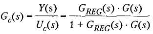
Obviously, the more parametersG REG (s), the more degrees of freedom the regulator has. By adjusting these parameters, the behavior of the transfer function of a closed system can, if desired, be varied within a fairly wide range. Further, the level of complexity of the regulator required to achieve the specified characteristics is discussed.
Proactive Control by Reference Value
The simplest control system reacts only to an errore (t) and does not use two separate inputs separately ?? reference value and process output parameter.
However, an error can occur for two reasons, one of which ?? change of reference or reference signalu c (t), and the second ?? change in load or some other disturbance in the system that causes a change in the output signaly (t). Changing the reference value ?? this is a well-known outrage. If the controller can use the relevant information, does this generally improve the characteristics of the closed system? physical process and regulator. In this senseproactive management.
Consider the regulator [equation (6.4)], which consists of two parts. Feedback loopGp B (s) is the initial regulator,e. The so-called anticipation loopG FF (s) controls the changes in the reference value and adds a correction term to the control signal so that the entire system reacts more quickly to changes in the reference signal (Figure 6.3). That is, the process controlling signalU (s) is the sum of two signals
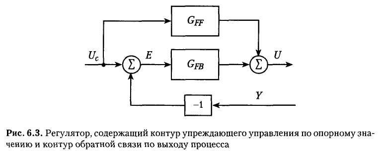
This expression can be rewritten in the form
where U Fi ?? pre-emptive signal by reference value (setting action),a Upg ?? feedback signal. The controller has two input signalsU c (s) and Y (s) and, therefore, can be described by two transfer functionsGp ^ (s) and G ^ (s) (Figure 6.4).
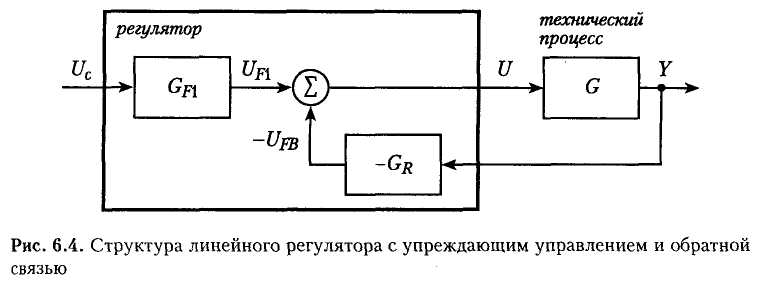
This expression can be transformed as follows
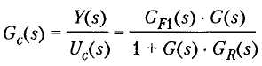
Since the controller corresponding to equation (6.4) has more adjustable coefficients than the simplest controller of equation (6.3), it is reasonable to assume that the closed system has better characteristics. The transfer function of the complete control loop can be obtained from Fig. 6.4.
The position of the poles of the feedback system can be changed using the controllerG R (s), and a pre-emptive regulatorG Fi (s) adds new zeros to the system. It follows that the entire system can respond quickly to changes in the reference signal, ifG F y (s) is properly selected.
Proportional-integral-differential(PID) controller ?? The most common structure of the regulator in process control and servomechanisms. Therefore, it will be discussed in detail in the next few sections.
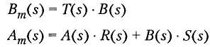
Parameters of polynomialsR (s), S (s), and T (s) can be chosen in such a way that
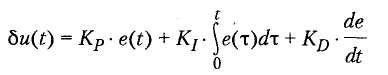
The PID controller generates an output signal that is the sum of three proportional control components, regulation by integraland regulation by the derivative. First partUp (t) is proportional to the error of the output quantity, i.e., the difference between the output quantity and the reference value, the second partUj (t) ?? integral with respect to the error time of the output quantity, and the third partu D (t) ?? the error derivative.
The equation of the classical PID controller has the form
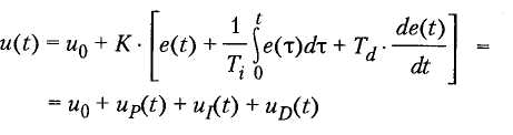
The parameter K ?? regulator gain, T i ?? integration time constant, and T d ?? differentiation time constant. The coefficient U 0 is adjustment valueor offset, adjusting the average level of the output signal of the regulator.
Some controls, especially older models, instead of amplifying, have a settingbands of proportionality, which is defined asRV = 100 / K and is usually expressed as a percentage. This definition is valid only ifK is dimensionless.
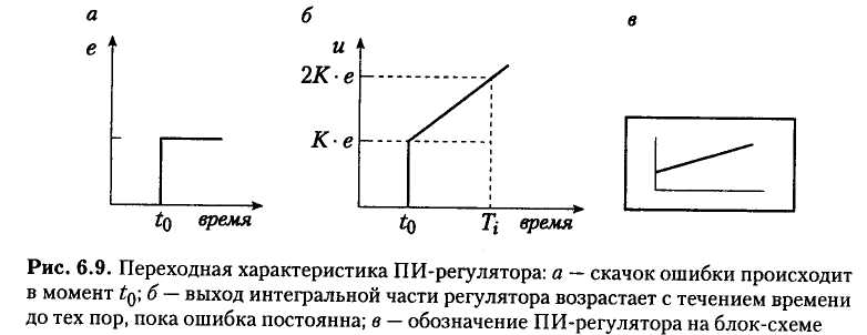
Integral time constantT i is present in the denominator of equation (6.12)? Thus, the values of the individual terms of the regulator equation turn out to be commensurable. Confirmation of this is clearly seen from the transient characteristic of the proportional-integrating (PI) regulator. Immediately after the error jumpe (t) at the output of the regulator, we haveK * e. As time passesT i the output value of the regulator becomes twice as large (Figure 6.9). The PI controller is often symbolically represented by its transient response.
The regulator can also be described using the Laplace transform. Applying it to the equation (6.12), we obtain
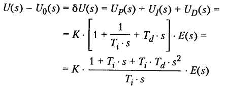
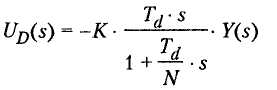
where E (s) ?? laplace images for signal componentsu p (t), u I (t), and u D (t) respectively. The degree of the numerator exceeds the degree of the denominator, so the gain of the regulator tends to infinity at high frequencies ?? this is a consequence of the differential component. In practice, differentiation can not be performed accurately, so a first-order approximation with a time constantT D and the PID controller equation takes the form
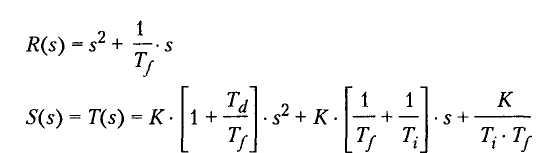
The PID controller is a special case of the generalized regulator [equation (6.7)] and can be expressed in terms of polynomialsR, S and T. Equation (6.14) can be rewritten in the form
As a result, we get a PID controller
In fact, most technical processes are of order higher than the second, but PID regulators can often be successfully used to manage such processes. This is due to the fact that many processes that actually have higher-order dynamics behave approximately like second-order systems. In systems that can not be approximated by second-order equations, the use of PID regulators is not recommended. In particular, this refers to mechanical systems having several vibrational components of motion.
Other types of PID parameterization
In many cases, the PID controller is parameterized in accordance with the following equation
This parametrization is equivalent to equation (6.12). However, there is an important practical limitation, because of which equation (6.18) can not be applied universally. The amplification of the entire "classical" PID controller [equation (6.12)] can be changed with a single parameterTO, which is very convenient, in particular, when starting or adjusting the technical process. This effect is also evident from the logarithmic frequency response. The classical regulator under changeTO the entire characteristic is displaced vertically, and its shape remains unchanged. In other words, the gain varies the same for all frequencies. In the parametric form (6.18), for any modification of the parameters, not only the gain, but also the fracture points of the individual segments of the logarithmic frequency characteristic changes.
Do the ideal controller have three parameters ??K, 7 J - and 7 ^ ?? can be customized individually, however in practice, if the regulator is manufactured using analog technology, individual control modes usually affect each other. This influence can be so significant that the actual and nominal values of the parameters will differ by 30%. In digital control systems, the controller parameters can be adjusted with the required accuracy, and their mutual influence is absent.
Implementing the PID controller
When implementing the regulator, it is necessary to take into account many different factors. First of all, we need to develop a discrete model of the regulator and determine the corresponding sampling frequency. The amplitude of the output value of the regulator must be "realistic", ie, be between the minimum and maximum allowable values. This limitation causes additional problems in the implementation and operation. In many applications, not only the output signal must be limited, but also the rate of its change due to the physical capabilities of the actuators and preventing their excessive wear. Changing parameter settings and switching from automatic operation to manual or other changes in operating conditions should not lead to disturbances in the regulated process. All these problems are discussed in this section.
Regulators can be created by analog technology based on operational amplifiers or, which is becoming more common, as digital devices based on microprocessors. Do they have almost the same appearance? the regulator is enclosed in a small, robust housing that allows installation in an industrial environment.
Discrete PID controller model
In order for the analog controller to be implemented programmatically, its discrete model is needed. For this, the same methods as described in Section 5.4 for low-frequency and high-frequency analog filters and their conversion to digital filters are used.
If the regulator is initially projected on the basis of an analog description and then its discrete model is constructed, for sufficiently small sampling intervals, the time derivatives are replaced by finite differences, and the integration? summation (Section 3.4). This approach will be used in this case.
The error of the output value of the process [equation (6.1)] is calculated for each sample
![]()
It is assumed that the sampling intervalh is constant. Any signal changes that might occur during the sampling interval are not taken into account (Sections 5.1.3 and 5.1.4).
There are two types of controller algorithm ?? position and increments.
The position algorithm
AT positional algorithmthe output signal is the absolute value of the control variable of the actuator. The discrete PID controller has the form
Even with zero control error, the output signal is non-zero and is determined by the offsetu 0.
In accordance with equation (6.14), the proportional part of the regulator has the form
![]()
The integral is approximated by finite differences
with a constant
The value of the second term for smallh and large T , - can become very small, so care must be taken to ensure the necessary accuracy of its machine representation.
The differential part of the PID controller is obtained from (6.17) by substituting the expression (6.15)
The corresponding differential equations connectinguj (t) and y (t), have the form
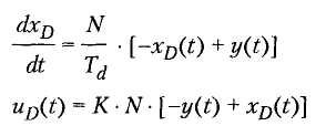
where Xp (t) is introduced as a state variable (this can be verified by applying the Laplace transform to equations (6.25) and (6.26) and eliminatingX £, (t)). The derivative in equation (6.25) is approximated by the difference back
where
![]()
It should be noted that the backward difference approximation is numerically stable for anyT d. The differential part of the PID controller can be represented as
Determining the sampling frequency in control systems
Determining an adequate sampling frequency for the management process is a non-trivial task and can rather be considered an art than a science. Too low sampling frequency can reduce the effectiveness of control, especially the ability of the system to compensate for disturbances. However, if the sampling interval exceeds the reaction time of the process, the disturbance can affect the process and disappear before the regulator initiates a corrective action. Therefore, when determining the sampling frequency, it is important to take into account both the dynamics of the process and the characteristics of the disturbance.
On the other hand, the sampling frequency should not be too high, as this will lead to increased computer load and deterioration of the actuator. Thus, determining the sampling frequency represents a trade-off between the requirements of the dynamics of the process and the available performance of the computer and other technological mechanisms. Standard digital controllers that operate with a small number of control loops (from 8 to 16) use a fixed sampling frequency on the order of fractions of a second.
The sampling frequency is also affected by the signal-to-noise ratio. For small values of this ratio, that is, for large noise, a high sampling frequency should be avoided, because the deviations in the measurement signal are more likely associated with high-frequency noise, rather than with real changes in the physical process.
The main task of primary signal processing is to digitize it and then restore it in a set of discrete values. The discretization theorem does not take into account the duration of the calculations for signal reconstruction, and in theory this time can be infinite. Moreover, the signal analyzed by this theorem is considered to be periodic, and in real control systems this is usually not the case. These factors also affect the sampling frequency.
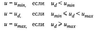
Control signal limitation
The output of the controller must have a limited amplitude for at least two reasons. First, the amplitude of the output signal can not exceed the range of the DAC at the output of the computer; secondly, the operating range of the actuator is always limited. The valve can not be opened more than 100%, the motor can not be supplied with unlimited current and voltage. Therefore, the control algorithm must include some function that limits the output signal.
In some cases, it should be determinedzone of insensitivity,or dead zone. If a regulator with an incremental algorithm is used, the changes in the control signal can be so small that the actuator can not process them. If the control signal is sufficient to act on the actuator, it is advisable to avoid small but frequent trips that can accelerate its wear. A simple solution is to sum the small changes in the control variable and give the control signal to the actuator only after a certain threshold value has been overcome. Of course, the deadband zone makes sense only if it exceeds the resolution of the DAC at the output of the computer.
Prevention of integral saturation
Integral saturation(integral windup) is the effect that is observed when the PI - or PID controller for a long time should compensate for an error outside the range of the controlled variable. Since the output of the regulator is limited, it is difficult to reduce the error to zero.
If the control error persists for a long time, the value of the integral component of the PID controller becomes very large. In particular, this occurs if the control signal is limited enough that the calculated output of the regulator is different from the actual output of the actuator. Since the integral part becomes zero only a short time after the error value has changed the sign, the integral saturation can lead to a large overshoot. Integral saturation is the result of non-linearities in the system associated with limiting the output control signal, and can never be observed in a truly linear system.
Let's consider the told on an example. The PI controller based on the positional algorithm is used to control the servomotor. The reference value for the angle of rotation of the motor axis changes so much that the output control signal saturates ?? voltage applied to the motor. In fact, the acceleration of the engine is limited. The transient characteristic of the angle of rotation of the motor axis is shown in Fig. 6.13.
One way to limit the influence of the integral part is in conditional integration. While the error is large enough, its integral part is not required for the formation of a control signal, but for controlling a sufficiently proportional part. The integral part used to eliminate stationary errors is necessary only in cases where the error is relatively small. In conditional integration this component is taken into account in the final signal only if the error does not exceed a certain threshold value. For large errors, the PI controller acts as a proportional controller. Selecting a threshold for activating the integral member ?? Far from being a trivial task. In analog regulators, conditional integration can be performed using a Zener diode (limiter), which is connected in parallel with the capacitor in the feedback loop of the operational amplifier in the integrator block of the regulator. This scheme limits the contribution of the integral signal.
In digital PID controllers, integral saturation can be avoided in a more convenient way. The integral part can be adjusted at each sampling interval so that the output of the regulator does not exceed a certain limit. Control signalu d first it is calculated using the PI-regulator algorithm, and then it should be checked whether it exceeds the specified limits
After limiting the output signal, the integral part of the regulator is reset. Below is an example of a PI regulator program with protection against saturation ?? As long as the control signal remains within the specified limits, the last operator in the text of the program does not affect the integral part of the regulator.
To prevent saturation of the PID controller, the described method should be slightly modified. The integral part is updated with the valuee s. = and ?? uj, which is the difference between the actual current output of the actuatorand and the calculated output of the regulatorand. The output of the actuator is either measured directly, if possible, or calculated using a model. Errore s is zero if the actuator provides the required control signal and there is no saturation. To reset the integral part, the signale s multiplied by a factor of 1 / T, whereT t is a coefficient, which is calledtracking time constant. In the PI-regulator algorithm given above, this time constant ish, ie, the update of the output value of the regulator occurs already at the time of the next sample. If the controller algorithm contains a differential part, it is advisable to update the integral much more rarely. The corresponding value for the tracking time constantT t is equal to the integration time 71 , -. In this case, the output value of the PI controller is
where u ?? limited valueand [equation (6.34)]. If the control signal is saturated, the differenceu - u d will change the integral part until saturation disappears, that is, saturation is prevented. This method corresponds to Fig. 6.13at.
Differentiating the integral part, we obtain
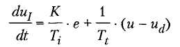
or in a discrete form
As a result, the PI controller algorithm becomes
where is determined from equation (6.35). In this case, the integration is approximated by the differences in front instead of the differences back. Such a replacement is necessary, sincemust be known before calculating the integral part.